Tutorial 07: Combining Multiple Molecules
Objectives
This tutorial will teach:
Rotation/translation of
Moleculeobjects.Direct creation and editing of
Moleculeobjects.
Overview
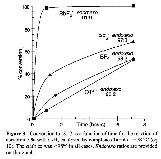
Metal triflates are frequently employed as “M+” precursors in Lewis-acid-catalyzed transformations, since the weakly-binding triflate can easily be displaced by Lewis-basic ligands. However, reported anion effects imply that “weakly-coordinating anions” like triflate may indeed have a non-negligible effect on catalysis. In one such study by Evans and coworkers, the counterion for a Cu(II)-tBuBox complex was found to have a dramatic effect on rate and lesser effects on enantioselectivity and diastereoselectivity, indicating that one or more equivalents of the counterion are present in the transition state:
Understanding how anions are bound to cationic catalysts could improve mechanistic understanding and lead to the design of improved catalytic systems. Computational modelling of weakly-bound ion pairs is difficult, however, because of the potential for numerous nearly degenerate binding modes. Accordingly, many distinct arrangements must be sampled and evaluated: although such an approach would be tedious by hand, automation with cctk renders it facile.
This tutorial will focus on evaluating the ground-state conformation of Evans’s system for the hexafluoroantimonate and triflate anions. We will make the simplifying assumption that only one anion will coordinate to the catalyst at a time, consistent with observation of singly-cationic metal–ligand complexes in solution.
Creating Structures
The structures of Cu(II)-tBuBox (S=1/2 dication), SbF6 (S=0 anion), and OTf (S=0 anion) were first optimized separately at the UB3LYP-D3BJ/6-31G(d)-SDD(Sb,Cu)/SMD(dichloromethane) level of theory.
In order to efficiently manipulate the ion pair, all molecules were loaded into cctk and then centered:
def center_molecule(molecule):
    """
    Moves a ``Molecule`` object's centroid to the origin
    """
    atoms = np.arange(0, molecule.num_atoms())
    molecule.translate_molecule(-molecule.geometry[atoms].mean(axis=0))
    return molecule

cation = center_molecule(GaussianFile.read_file("CuII-tBuBox-dication.out").get_molecule())
anion1 = center_molecule(GaussianFile.read_file("SbF6_anion.out").get_molecule())
anion2 = center_molecule(GaussianFile.read_file("OTf_anion.out").get_molecule())

anions = [anion1, anion2]
anion_names = ["SbF6", "OTf"]
To determine the relative position of the two molecules, a random vector was sampled from a spherical distribution:
def spherical_random(radius=1):
    """
    Generates a random point on a sphere of radius ``radius``.
    """
    v = np.random.normal(size=3)
    v = v/np.linalg.norm(v)
    return v * radius
The anion was then rotated randomly about all 3 Cartesian axes, and the atomic numbers and coordinates were concatenated to produce a new Molecule object.
The output structures were written to .gjf files:
for i in range(num_structures):
    trans_v = spherical_random(radius=8)
    for j in range(len(anions)):

        x = copy.deepcopy(anions[j])
        x.translate_molecule(trans_v)
        x.rotate_molecule(np.array([1,0,0]), np.random.random()*360)
        x.rotate_molecule(np.array([0,1,0]), np.random.random()*360)
        x.rotate_molecule(np.array([0,0,1]), np.random.random()*360)

        atoms = np.hstack((cation.atomic_numbers.T, x.atomic_numbers.T))
        geoms = np.vstack((cation.geometry, x.geometry))

        mx = Molecule(atomic_numbers=atoms, geometry=geoms, charge=1, multiplicity=2)
        GaussianFile.write_molecule_to_file(f"CuII-tBuBox-{anion_names[j]}_c{i}.gjf", mx, "#p opt b3lyp/genecp empiricaldispersion=gd3bj scrf=(smd, solvent=dichloromethane)", footer)
The complete script (generate_ion_pairs.py) looks like this:
import copy
import numpy as np
from cctk import Molecule, GaussianFile

num_structures = 25

footer = ""
with open('footer', 'r') as file:
    footer = file.read()

def spherical_random(radius=1):
    """
    Generates a random point on a sphere of radius ``radius``.
    """
    v = np.random.normal(size=3)
    v = v/np.linalg.norm(v)
    return v * radius

def center_molecule(molecule):
    """
    Moves a ``Molecule`` object's centroid to the origin
    """
    atoms = np.arange(0, molecule.num_atoms())
    molecule.translate_molecule(-molecule.geometry[atoms].mean(axis=0))
    return molecule

cation = center_molecule(GaussianFile.read_file("CuII-tBuBox-dication.out").get_molecule())
anion1 = center_molecule(GaussianFile.read_file("SbF6_anion.out").get_molecule())
anion2 = center_molecule(GaussianFile.read_file("OTf_anion.out").get_molecule())

anions = [anion1, anion2]
anion_names = ["SbF6", "OTf"]

for i in range(num_structures):
    trans_v = spherical_random(radius=8)
    for j in range(len(anions)):

        x = copy.deepcopy(anions[j])
        x.translate_molecule(trans_v)
        x.rotate_molecule(np.array([1,0,0]), np.random.random()*360)
        x.rotate_molecule(np.array([0,1,0]), np.random.random()*360)
        x.rotate_molecule(np.array([0,0,1]), np.random.random()*360)

        atoms = np.hstack((cation.atomic_numbers.T, x.atomic_numbers.T))
        geoms = np.vstack((cation.geometry, x.geometry))

        mx = Molecule(atomic_numbers=atoms, geometry=geoms, charge=1, multiplicity=2)
        GaussianFile.write_molecule_to_file(f"CuII-tBuBox-{anion_names[j]}_c{i}.gjf", mx, "#p opt b3lyp/genecp empiricaldispersion=gd3bj scrf=(smd, solvent=dichloromethane)", footer)
Analyzing Structures
The above script was used to create 25 unique conformations of both the OTf and SbF6 complexes, which were optimized in Gaussian 16.
Successfully converged jobs were then resubmitted (using scripts/resubmit.py) with the following input line:
#p opt pop=hirshfeld b3lyp/genecp empiricaldispersion=gd3bj scrf=(smd, solvent=dichloromethane)
After several days, 37 out of the 50 starting structures had converged and were selected for further analysis.
The analysis script (scripts/analyze.py) was modified by addition of the following lines:
cation_anion_dist = 0
mul_q = 0
hir_q = 0
if 29 in mol.atomic_numbers:
    mul_q = float(parse.find_parameter(lines, "    52  Cu", 4, 2)[-1])
    hir_q = float(parse.find_parameter(lines, "    52  Cu", 8, 2)[-1])

    if 16 in mol.atomic_numbers:
        cation_anion_dist = mol.get_distance(52, 54)
    elif 51 in mol.atomic_numbers:
        cation_anion_dist = mol.get_distance(52, 53)
The output data were written to a .csv file, read into Python and analyzed using Pandas.
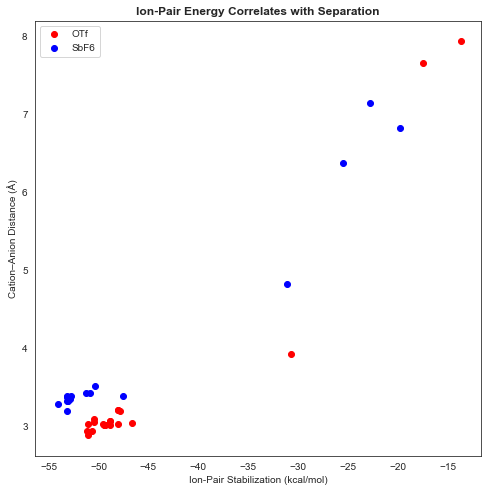
As expected, closer anion–cation complexes were found to be substantially more stable (all energies relative to infinitely separated cation and anion):
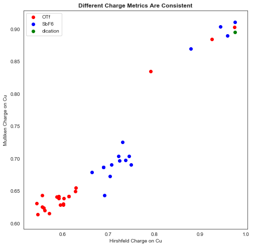
Copper charges calculated by the Mulliken and Hirshfeld schemes correlated very well, which was encouraging:
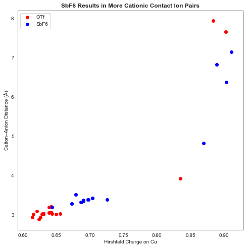
An analysis of charge versus cation–anion distance showed a clear discrepancy between OTf and SbF6 complexes: OTf complexes generally bound more tightly and resulted in a less cationic Cu center. (A small proportion of anions ended up “trapped” behind the ligand, resulting in very large cation–anion distances and high-energy complexes).
Visualization of the lowest-energy OTf- and SbF6-bound structures reveals that both are coordinated to the Cu center in an inner-sphere fashion, despite SbF6 generally being considered a “non-coordinating” anion:
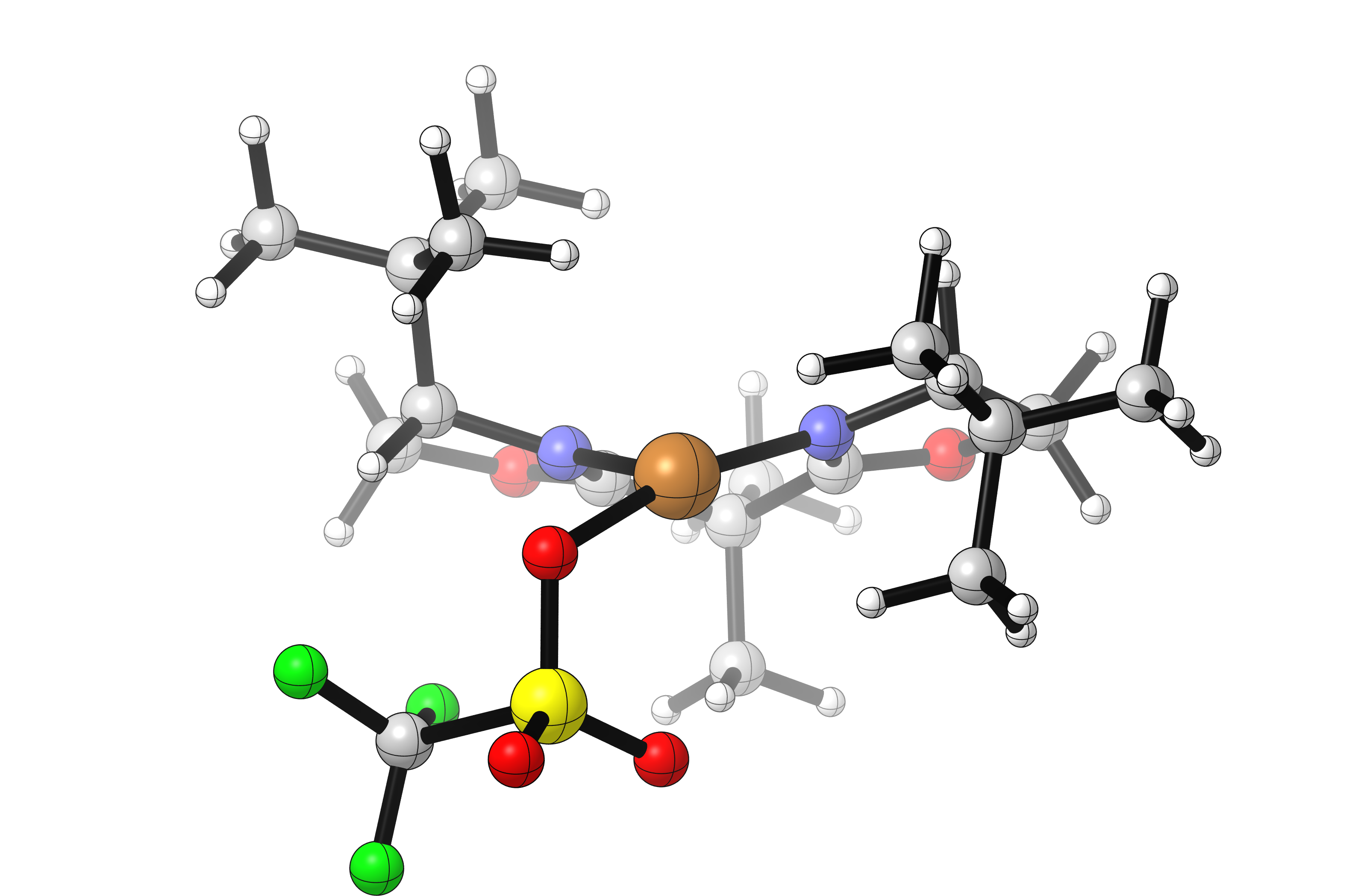
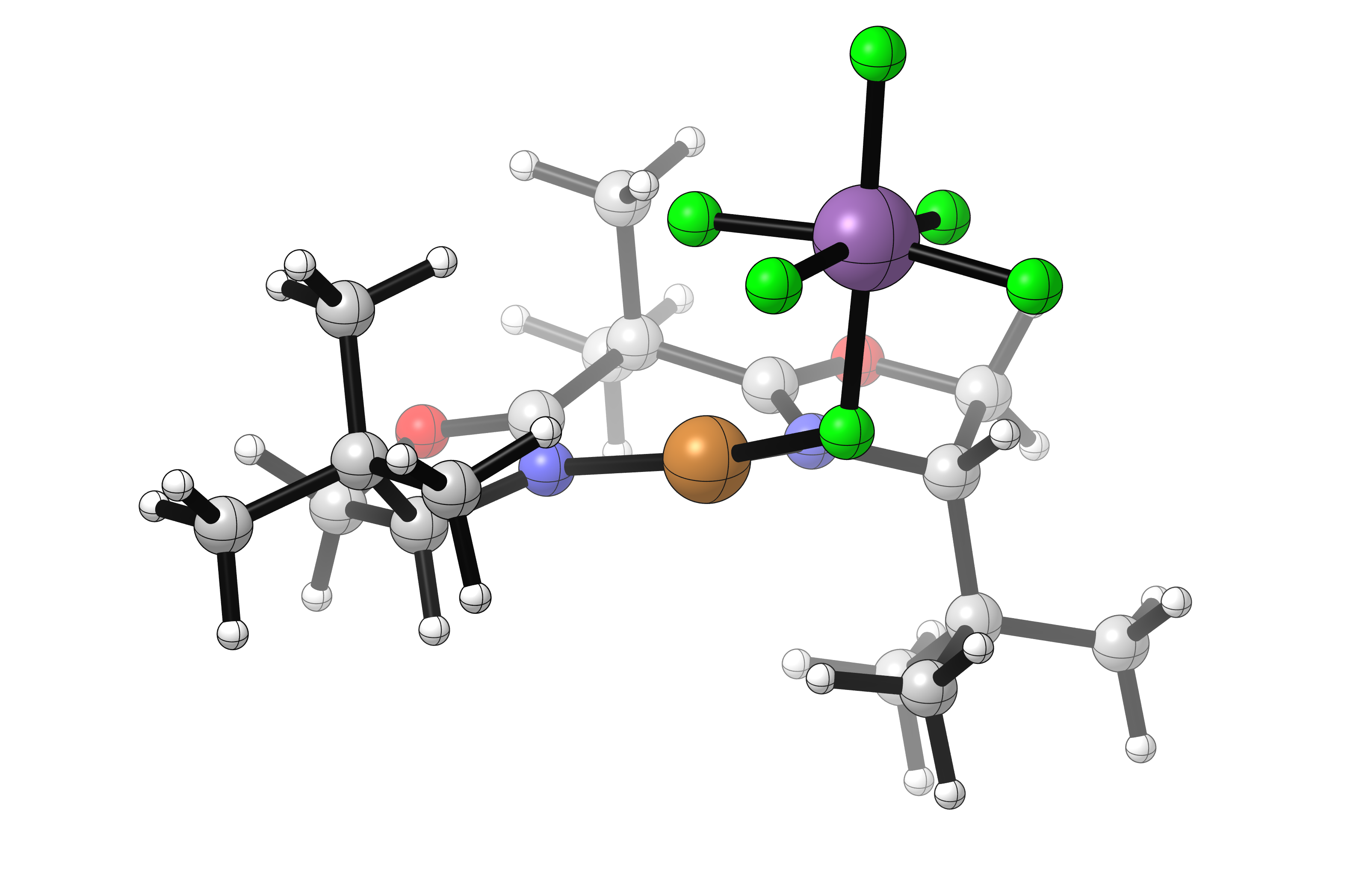
In this case it seems that the more diffusely anionic SbF6 anion results in a more weakly-bound complex with a more cationic copper. This complex could either react directly with substrate, or exist in equilibrium with a solvent-separated ion pair which could itself react with substrate. Either scenario is consistent with the observed rate increases using SbF6.
A more in-depth study might examine free energy and potential of mean force in explicit solvent, as well as investigating substrate approach with a variety of anion geometries.