Reading and Writing ORCA Files¶

import cctk is assumed.
cctk was originally designed with Gaussian in mind, but supports basic writing of ORCA input files and parsing of ORCA output
The default print level in ORCA ! NormalPrint is recommended for parsing with cctk
Note that ! MiniPrint may make Orca output files unreadable by cctk

Writing a simple ORCA input file¶

In this recipe, we convert an .xyz file into an ORCA .inp file.
cctk can only write single-geometry input files for ORCA

read_path = "test/static/test_peptide.xyz"
path = "test/static/test_peptide.inp"
file = cctk.XYZFile.read_file(read_path)

header = "! aug-cc-pVTZ aug-cc-pVTZ/C DLPNO-CCSD(T) TightSCF TightPNO"
variables = {"maxcore": 4000}
blocks = {"pal": ["nproc 4"], "mdci": ["density none"]}
cctk.OrcaFile.write_molecule_to_file(path, file.get_molecule(), header, variables, blocks)

The parent .xyz is test_peptide.xyz.
The resulting .inp is test_peptide.inp.

Writing an ORCA input file from a SMILES string¶

In this recipe we use the SMILES string of uridine to quickly generate an input file for geometry optimization and frequency calculation.
Writing molecules from SMILES requires RDKIT which can be installed with pip install rdkit

write_path = "test/static/orca_uridine_opt_freq.inp"

# define a smiles string
SMILES = "C1=CN(C(=O)NC1=O)C2C(C(C(O2)CO)O)O"

# define a cctk molecule from SMILES string
mol = cctk.Molecule.new_from_smiles(SMILES)

cctk.OrcaFile.write_molecule_to_file(write_path, mol,
        header="! b3lyp/G 6-31g(d) D3 CPCM(water) opt freq tightscf")

This writes orca_uridine_opt_freq.inp.

Reading Output of ORCA Geometry Optimization¶

Submission of the example input above returns: orca_uridine_opt_freq.out

Warning: parsing of dipole_moment, mulliken_charges, and lowdin_charges is not fully supported for relaxed scan jobs.

To access properties of the final structure in the geometry optimization:

path = 'test/static/orca_uridine_opt_freq.out'
file = cctk.OrcaFile.read_file(path)

# to access a property from the final structure, we use tuple indexing
# where `-1` represents the final structure
energy = file.ensemble[-1, 'energy']
# returns -911.091006238863

# to access the all the properties for the final structure
properties = file.ensemble.properties_list()[-1]
# returns a dictionary of all accessible properties and their values for the final structure
# {'energy': -911.091006238863,
# 'filename': './test/static/orca_uridine_opt_freq.out',
# 'iteration': 60,
# 'scf_iterations': 6.0,
# 'frequencies': [41.02, 60.16, 64.69, 106.05, ...]
# 'enthalpy': -910.84749131,
# 'gibbs_free_energy': -910.90399464,
# 'temperature': 298.15,
# 'quasiharmonic_gibbs_free_energy': -910.902280867151,
# 'mulliken_charges': OneIndexedArray([-0.274128,  0.092336, -0.455099, ...]),
# 'lowdin_charges': OneIndexedArray([-0.21586 , -0.015003, -0.018213, ...]),
# 'dipole_moment': 5.04114}

To access the final geometry in the ensemble:

mol = file.ensemble.molecule_list()[-1]

#equivalently
mol = file.get_molecule()
# or
mol = file.get_molecule(-1)

# We can then do something with that geometry
# For example, use it to write an input for a single point calculation

write_path = "test/static/uridine_sp.inp"
header = "! aug-cc-pVTZ aug-cc-pVTZ/C DLPNO-CCSD(T) TightSCF TightPNO"
variables =  {"maxcore": "4000"}
blocks = {"mdci": ["density none"], "pal": ["nproc 8"] }
cctk.OrcaFile.write_molecule_to_file(write_path, mol, header, variables, blocks)

Which writes the file uridine_sp.inp

We can also access the properties of all geometries in the ensemble with:

file.ensemble.properties_list()
# returns a list of dictionaries
# each dictionary in the list corresponds to a geometry from the optimization
# each dictionary contains property keys mapped to property values for the specified geometry.

To access a given property for each member of the ensemble:

geom_iters = file.ensemble[:,'iteration']
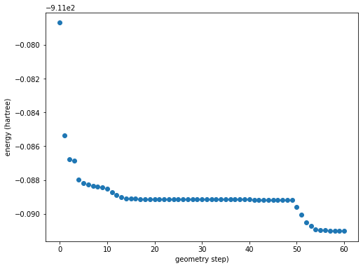
energy = file.ensemble[:, 'energy']
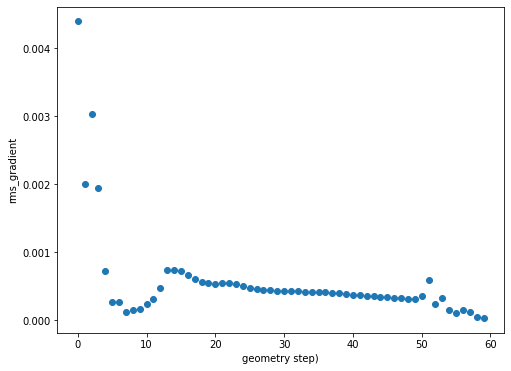
rms_grad = file.ensemble[:, 'rms_gradient']

We can then plot the property as a function of optimization step:

import matplotlib.pyplot as plt

energy_figure = plt.figure(figsize=(8,6))
plt.scatter(geom_iters, energy)
plt.ylabel(f"energy (hartree)")
plt.xlabel(f"geometry step")
plt.close()

rms_grad_figure = plt.figure(figsize=(8,6))
plt.scatter(geom_iters, rms_gradient)
plt.ylabel(f"rms_gradient")
plt.xlabel(f"geometry step")
plt.close()

Calling energy_figure returns:

Calling rms_grad_figure returns: